Format cells
Bold and colour cells, align text, set number and date formats, add notes and colour cells automatically with conditional formatting.
Make a sheet readable: bold and colour cells, align text, choose how numbers and dates look, add notes, and colour cells automatically with conditional formatting.
Before you start: Can edit on Sheets. Formatting is saved with the sheet, so everyone sees it.
Text and colour
Select cells, then use the toolbar:
| Button | What it does |
|---|---|
| Bold, Italic, Underline, Strikethrough | Toggle the style. Ctrl + B, Ctrl + I, Ctrl + U also work. |
| Text colour | Automatic or one of Red, Orange, Yellow, Green, Teal, Blue, Purple, Pink, Gray. |
| Fill colour | No fill or one of the same colours. |
| Align left, Align centre, Align right | Horizontal alignment. Numbers align right unless you choose otherwise. |
| Wrap text | Lets long text run onto a second line inside the cell. |
| Clear formatting | Removes styles from the selected cells. Values stay. |
The colours are chosen to stay readable in both light and dark mode.
Number and date formats
Click 123 (Number format) on the toolbar. The choice applies to the whole column of the selected cell.
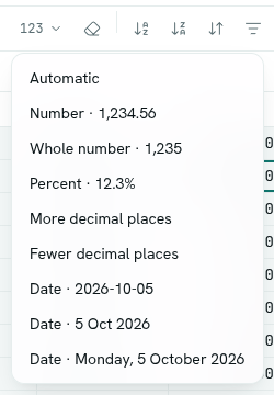
| Option | Example |
|---|---|
| Automatic | As typed |
| Number | 1,234.56 |
| Whole number | 1,235 |
| Percent | 12.3% (0.123 shows as 12.3%) |
| More decimal places / Fewer decimal places | One more or one fewer digit |
| Date | 2026-10-05, 5 Oct 2026, or Monday, 5 October 2026 |
Formats change only how values look. Formulas still use the full value.
Notes
- Select a cell and click Note on the toolbar (or right-click › Insert note).
- Type the Note (up to 1,000 characters) and save.
A cell with a note shows a small marker in its top-right corner. Hover the cell to read it. Right-click › Edit note changes it; Remove note deletes it.
Conditional formatting
Colour cells automatically from their value — for example every "Overdue" in red.
- Select the cells the rule should cover (for example the Status column).
- Click Conditional formatting on the toolbar.
- Click Add rule.
- Check the cells under Applies to, or click Use current selection.
- Under Format cells if, pick a condition: Greater than, Greater than or equal to, Less than, Less than or equal to, Equal to, Not equal to, Between, Text contains, Is empty or Is not empty. Fill in Value (and And for Between).
- Choose the look: Text colour, Fill and Bold.
- Click Done, then Save.
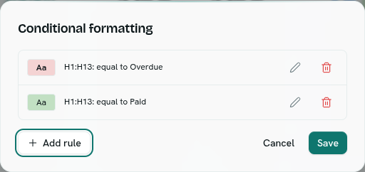
- The list shows each rule with a preview. Use the pencil to edit a rule and the bin to delete it.
- When several rules match a cell, the first one in the list wins.
- Rules follow the value: when "Open" becomes "Overdue", the colour changes on its own.
- A sheet can have up to 50 rules.
Tips
- Use bold and a fill colour on a header row, then freeze it (Freeze › Freeze 1 row).
- Conditional colours beat colouring by hand: they stay right as data changes.