Summarize data with pivot tables
Turn a long list of rows into a compact summary — totals, counts and averages by category — that refreshes from your data.
A pivot table turns a long list — sales, expenses, stock movements — into a summary you can read at a glance: one row per category, the figures you care about beside it, and a grand total at the bottom.
Before you start: you need permission to edit the workbook. Your data should have a header row (for example Region, Product, Amount) with one record per row below it.
Create a pivot table
- Open the workbook in Sheets and select your data, headers included. To use the whole sheet, just click any single cell.
- In the toolbar, choose Pivot table. The pivot table panel opens on the right.
- Leave First row is headers ticked if your first row holds column names.
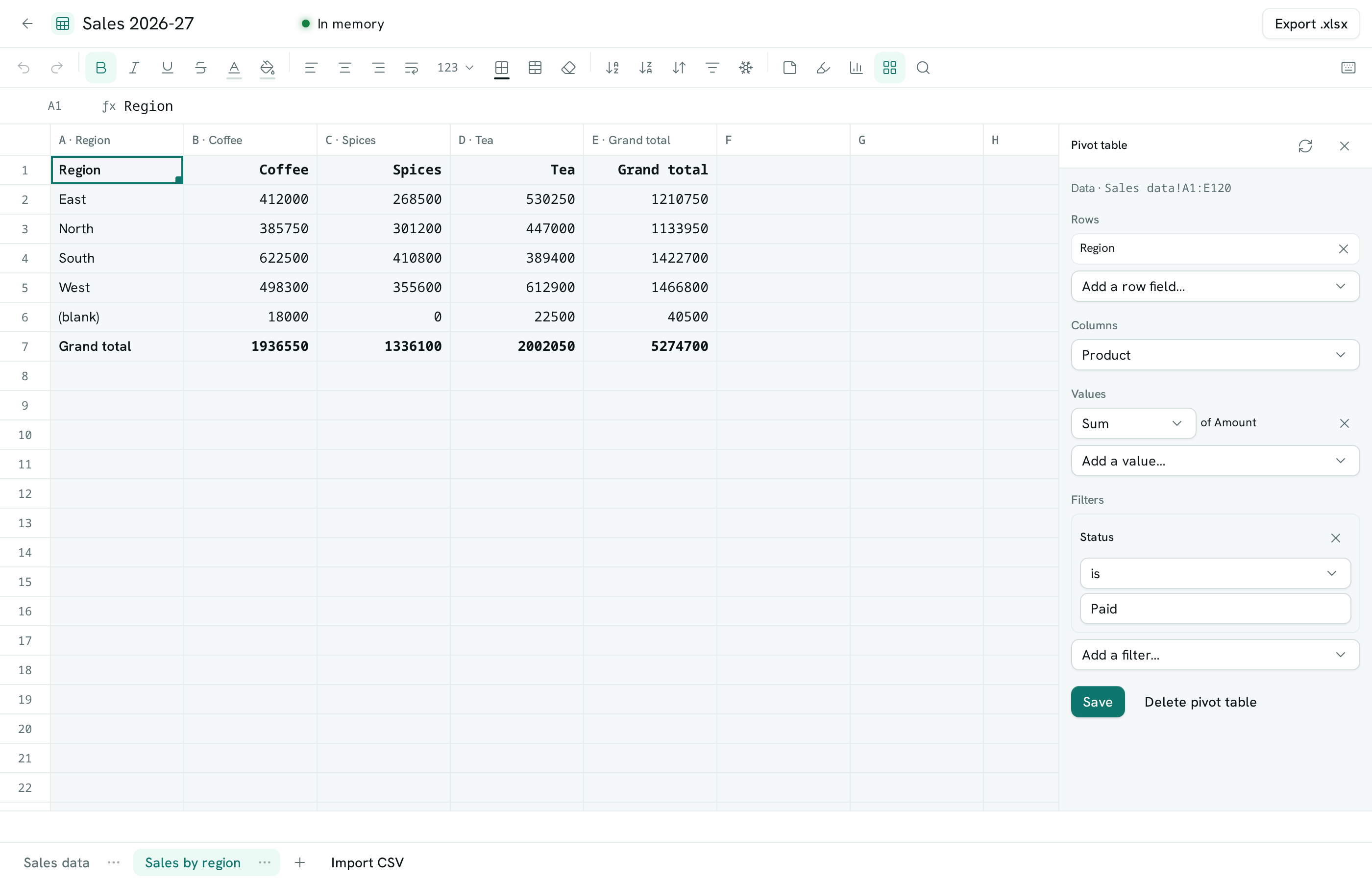
- Under Rows, pick the field to group by — for example Region. Add more row fields to break groups down further (for example Region, then Product).
- Optionally, under Columns, pick a field to spread across the top — for example Month.
- Under Values, pick what to summarize — for example Amount — and choose how: Sum, Count, Unique count, Average, Min or Max. You can add several values.
- Optionally, under Filters, pick a field and a condition (for example Status is
Paid) to include only matching rows. - Under Put it on, choose New sheet, or Existing sheet and the top-left cell where it should start.
- Choose Create pivot table.
The pivot table appears with bold headings, one row per group and a Grand total row. With a column field, each column value gets its own column and a Grand total column sits on the right.
Change a pivot table
- Open the sheet that holds the pivot table and choose Pivot table in the toolbar.
- Add or remove row fields, change the column field, values or filters.
- Choose Save. The pivot table is rebuilt in place.
Keep it up to date
A pivot table refreshes from its data every time you open its sheet. To refresh while you work, open the pivot table panel and choose the Refresh button at the top.
Remove a pivot table
- Open the sheet that holds it and choose Pivot table in the toolbar.
- Choose Delete pivot table and confirm. Its cells are cleared; the data it summarized is not touched.
Good to know
- Totals are exact to the paisa — amounts are added as decimals, never rounded along the way.
- Count counts filled-in cells; Unique count counts different values. Sum, Average, Min and Max use only cells holding numbers.
- Empty categories are listed as (blank), at the end.
- The cells of a pivot table are its own: you can't type over them. Change the pivot table from its panel instead. You can still write next to it, and you can point formulas and charts at its cells.
- A pivot table never writes over your cells. If it would grow into cells that already hold something, it stops and tells you which cell is in the way.
- A pivot table can hold up to 5,000 cells and spread up to 100 different values across its columns. Add a filter or pick fewer fields for bigger data.
- People who can only view the workbook see the pivot table as it was last refreshed.
- Rows are listed in one table with every group named on each line; there are no subtotal rows.
- When you download the workbook as Excel, the pivot table comes across as a summary of values.